Global Overlays
The Overlays menu in the sidebar allows you to view additional geographic information on your map.
Introduction
The World Climate refers to climate change as the study of the interactions between “temperature and energy, atmospheric composition, ocean and water, and the cryosphere” Global Climate Observing System (GCOS). Global climate change therefore refers to the fluctuation of these climate conditions and interactions over an extensive period, traditionally averaged over a 30-year period, although more recently 10-year and 5-year averaged periods have been used.
This user guide will take you through an overview of the data, the method behind the creation of the map products, and their various potential uses.
Data
Two key climate parameters are used to create Digimap for School’s World Climate overlays.
- Temperature
- Precipitation
The intention is to use downscaled, gridded files of averaged climate parameters over 30-year and 10-year periods to reconstruct a timeline of global climate change. The original formats are produced at 30-second resolution, although alternative downscaled datasets are made available through aggregation International Journal of Climatology. For the purposes of our study, all layers were produced using the 2.5 minutes resolution datasets. A summary table highlighting the information of each of the individual layers used for map creation is available in Table 1. All layers adopt a global land coverage, except in the 2010-2018 and 2020-2029 precipitation layers where Antarctica is omitted. These layers are displayed in WGS84.
Table 1
Summary table of the metadata of the product layers:
| Climate Parameter* | Year | Spatial Resolution | Source | |
|---|---|---|---|---|
| Temperature (°C) | 1970-2000 | GeoTIFF | 2.5 minutes | (Fick and Hijmans, 2017) |
| Temperature (°C) | 2010-2018 | GeoTIFF | 2.5 minutes | CRU-TS 4.03 (Harris et al., 2020) downscaled with WorldClim 2.1 (Fick and Hijmans, 2017) |
| Temperature (°C) | 2021-2040** | GeoTIFF | 2.5 minutes | CMIP6 (Eyring et al., 2016) downscaled with WorldClim 2.1 as |
| baseline climate (Fick and Hijmans, 2017) | ||||
| Precipitation (mm) | 1970-2000 | GeoTIFF | 2.5 minutes | (Fick and Hijmans, 2017) |
| Precipitation (mm) | 2010-2018 | GeoTIFF | 2.5 minutes | CRU-TS 4.03 (Harris et al., 2020) downscaled with WorldClim 2.1 (Fick and Hijmans, 2017) |
| Precipitation (mm) | 2020-2029 | GeoTIFF | 2.5 minutes | CMIP6 (Eyring et al., 2016) downscaled with WorldClim 2.1 as |
| baseline climate (Fick and Hijmans, 2017) |
* Calculated as averages over the indicated time period unless stated otherwise. ** Calculated as average minimum and maximum temperatures.
Creation
Due to the pre-processed (downscaled) nature of the datasets, all of the layers were readily available for use. These are viewable through GIS, and in producing a single layer for each climate parameter the monthly averages were combined. The visualisation methods were adopted in line with advice from an IPCC supporting document, the IPCC Visual Style Guide for Authors.
Symbology
For our map products, 14 subdivisions were used for the temperature layers and categorised using two contrasting hues; and 12 and 5 subdivisions used for precipitation using a single hue. The intention behind the usage of these colours attempts to connect diverging andnon-diverging datasets with intuitive cognition.
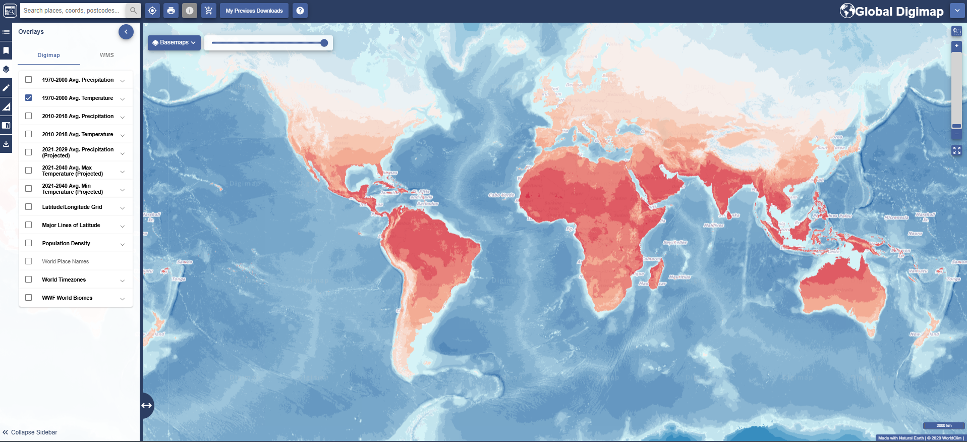
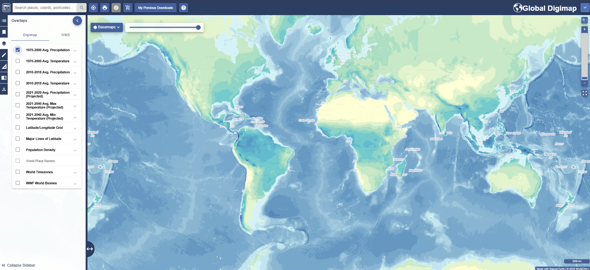
Two contrasting hues are chosen for the temperature layer pertaining to the negative/positive values. A single hue is appropriate for the precipitation layer to illustrate non-diverging data
Usage
The derived data products are available for use for a range of purposes including academic research, teaching and reuse for non-profit activities. The layers can be used individually per climate parameter or combined to offer a comprehensive understanding of global climate at a specific time period and/orto view changesrelative to previous or future datasets. The products can also be used for input into climate models for further analysis. In particular to the future climate datasets, these are modelled based on specific Socioeconomic Pathways (SSP), the Special Report on Emissions Scenarios (SRES) and climate models on CarbonBrief. In this case, an SSP2 scenario is selected for modelling temperature using the CNRM-CM6-1, and an SRES A2 scenario chosen to model precipitation using the CNRN-CM3. Briefly speaking, the former represents a “middle of the road” scenario where there are medium challenges presented to mitigation and adaptation to future socio-economic and technological trends. The latter refers to a state where countries are more oriented towards economic development amongst increasing population. Users should therefore be aware of the complexities and inherent degree of uncertainty to future climate modelling and of the limitations of these models in achieving this. These projections are predictive rather than conclusive.
Conclusion
This guide provides an explanatory overview of the global climate products available through DIGIMAP FOR SCHOOLS, the map creation processes and their various potential uses. The availability and geographicalscope of open data allowedfor the creation of global climate layers from 1970-2040 at high spatial resolution. The products allow for temporal and cross-country comparisons. Users are warned to use common sense in interpreting the future climate datasets – these are predictive as opposed to conclusive.
Licences
All data were licensed under the Creative Commons Attribution-ShareAlike 4.0 International Public License.
References
- GCOS, n.d. Global Climate Indicators. GCOS. Retrieved from: (https://gcos.wmo.int/en/global-climate-indicators).
- Hijmans, R.J., Cameron, S.E., Parra, J.L., Jones, P.G. and Jarvis, A., 2005. Very high-resolution interpolated climate surfaces for global land areas. International Journal of Climatology: A Journal of the Royal Meteorological Society, 25(15), pp.1965-1978.
- Gomis, M.I and Pidcok, R. (2018). IPCC Visual Style Guide for Authors. IPCC. Retrieved from: (https://www.ipcc.ch/site/assets/uploads/2019/04/IPCC-visual-style-guide.pdf).
- Hausfather, Z., 2018. Explainer: How ‘Shared Socioeconomic Pathways’ explore future climate change. Carbon Brief. Retrieved from: (https://www.carbonbrief.org/explainer-how-shared-socioeconomic-pathways-explore-future-climate-change).
- Nakicenovic, N. and Swart, R., 2000. Emissionsscenarios. Special report of the Intergovernmental panel on climate change.
Additional Dataset References
- Eyring, V., Bony, S., Meehl, G. A., Senior, C. A., Stevens, B., Stouffer, R. J., and Taylor, K. E.: Overview of the Coupled Model Intercomparison Project Phase 6 (CMIP6) experimental design and organization, Geosci. Model Dev., 9, 1937- 1958, doi:10.5194/gmd-9-1937-2016, 2016.
- Fick, S.E. and R.J. Hijmans, 2017. WorldClim 2: new 1km spatial resolution climate surfaces for global land areas. International Journal of Climatology 37 (12): 4302-4315.
- Harris, I.P.D.J., Jones, P.D., Osborn, T.J. and Lister, D.H., 2014. Updated high-resolution grids of monthly climatic observations–the CRU TS3. 10 Dataset. International journal of climatology, 34(3), pp.623-642.
- Hijmans, R.J., Cameron, S.E., Parra, J.L., Jones, P.G. and Jarvis, A., 2005. Very high-resolution interpolated climate surfaces for global land areas. International Journal of Climatology: A Journal of the Royal Meteorological Society, 25(15), pp.1965-1978